14 pts total
Problem # 1
Using this fake data set on lemur feeding rates do a two-factor ANOVA to determine whether feeding rate is influenced by sex and by the group each individual belongs to.
1 pt
A. Make a boxplot of feeding rate by sex
library(ggplot2)
theme_set(theme_bw(30))
lemurs <- read.table("../../static/datasets/lemurfeeding.txt", header=TRUE)
qplot(x=sex, y=feedingrate, data=lemurs, geom="boxplot", fill=sex)
## Warning: `qplot()` was deprecated in ggplot2 3.4.0.
## This warning is displayed once every 8 hours.
## Call `lifecycle::last_lifecycle_warnings()` to see where this warning was
## generated.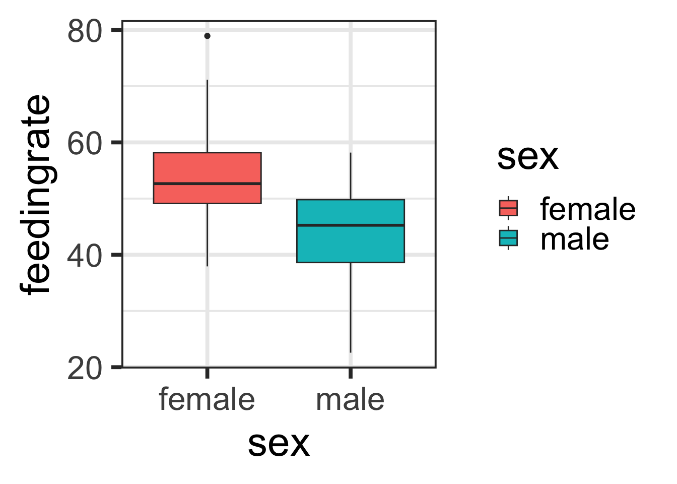
1 pt
B. Make a boxplot of feeding rate by group
qplot(x=group, y=feedingrate, data=lemurs, geom="boxplot", fill=group)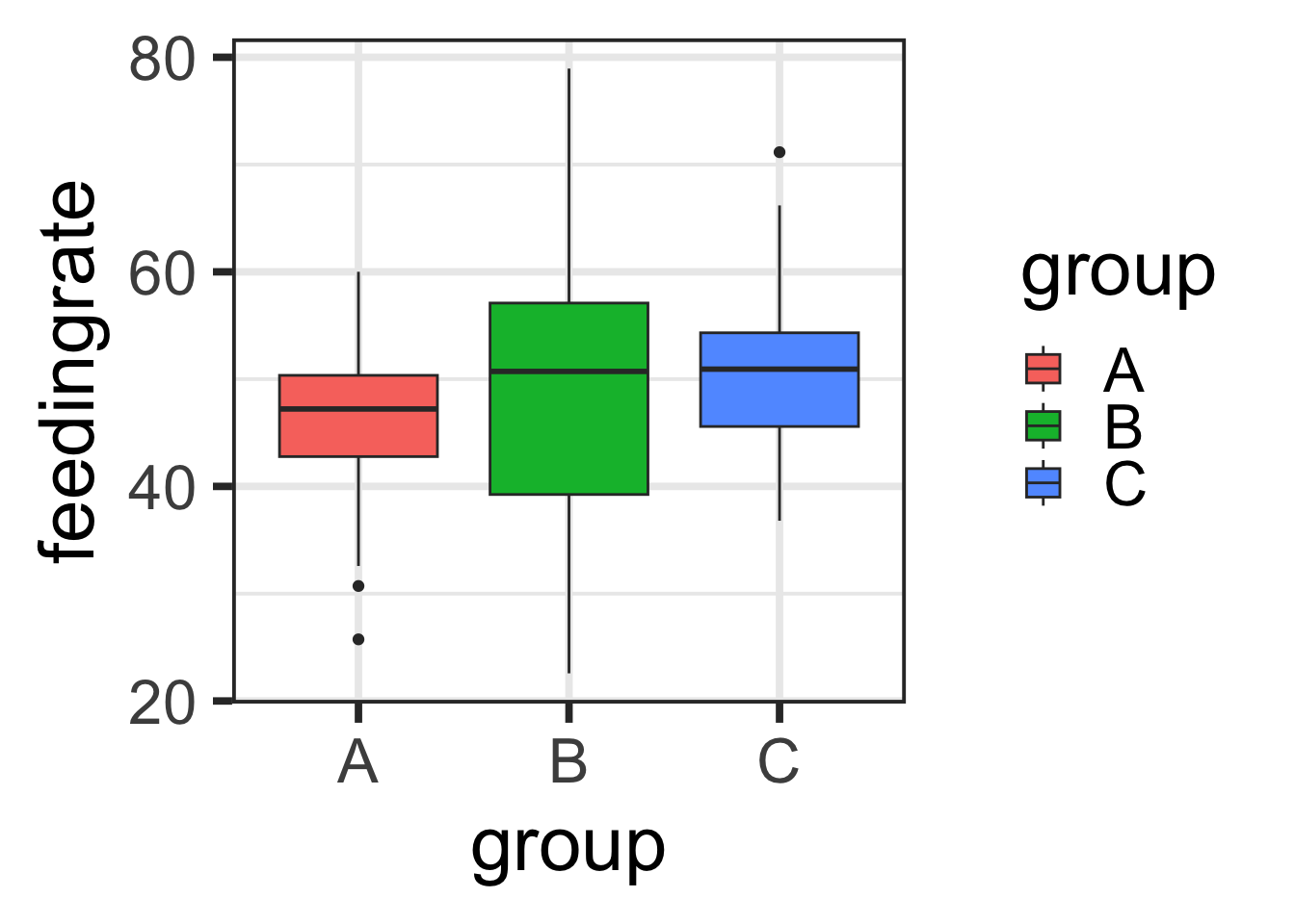
1 pt
C. Show the ANOVA table for the two way ANOVA with the interaction term.
anova(lm(feedingrate ~ group * sex, data=lemurs))## Analysis of Variance Table
##
## Response: feedingrate
## Df Sum Sq Mean Sq F value Pr(>F)
## group 2 467.7 233.85 4.5898 0.0121018 *
## sex 1 3077.2 3077.20 60.3967 3.732e-12 ***
## group:sex 2 1011.9 505.97 9.9307 0.0001057 ***
## Residuals 114 5808.3 50.95
## ---
## Signif. codes: 0 '***' 0.001 '**' 0.01 '*' 0.05 '.' 0.1 ' ' 12 pts
D. Explore the interaction between the two factors by creating a plot analogous to figure 10.3 (p 329) in the Gotelli book. Put the group on the X axis, and the mean feeding rate for each group on the Y axis (make this a line going across all factor levels). Color code the lines by sex.
library(dplyr)##
## Attaching package: 'dplyr'## The following objects are masked from 'package:stats':
##
## filter, lag## The following objects are masked from 'package:base':
##
## intersect, setdiff, setequal, uniongroupedLemurs <- lemurs %>% group_by(group, sex) %>% summarize(mean=mean(feedingrate))## `summarise()` has grouped output by 'group'. You can override using the
## `.groups` argument.qplot(x=group, y=mean, data=groupedLemurs, group=sex, geom="line", color=sex)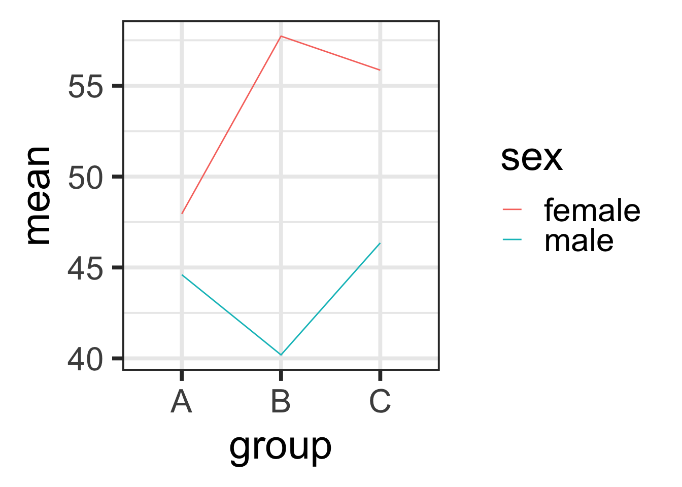
1 pt
E. Explain whether or not there is an interaction between the two factors.
Heck yeah there is. These lines are not parallel, so there is a non-additive interaction between sex and group.
Problem # 2
5 pts
Write a function to simulate ANOVA type data……
doANOVA <- function(sampleSize=20, grandMean=50, errorSD=5, meanDiff=3) {
  library(ggplot2)
  myError <- rnorm(sampleSize, mean = 0, sd = errorSD)
  groups <- rep(c("groupX", "groupY"), sampleSize/2)
  y <- grandMean + c((meanDiff/2)*-1, (meanDiff/2)) + myError
  print(qplot(x=groups, y=y, geom="boxplot"))
  myModel <- lm(y~groups)
  # Complicated way to calculate p yourself using pf() and degrees of freedom
  # p <- pf(summary(myModel)$fstatistic[1],
  #         summary(myModel)$fstatistic[2],
  #         summary(myModel)$fstatistic[3],
  #         lower.tail = FALSE)
  # easy way to get p from the ANOVA table
   p <- anova(myModel)[1,5]
  return(p)
}
3 pts
what effect do these parameters have on the p value?
- sample size - increasing n decreases the p value
- grand mean - no effect
- standard deviation of the error term - increasing error variance (sd) increases the p value