Homework #9 - Solution - Hompal Stats Class

10 pts total

Problem 1

A - 1pt

load this dataset on scapula morphology in Pan, Homo and Gorilla, and the Dikika fossil child. Details on this data can be found in Alemseged et al, 2006

scap <- read.table("https://stats.are-awesome.com/datasets/DIK-scap.txt", header=TRUE)

B - 1pt

Calculate the natural log of all the numeric variables

# log all the measurements, excluding the first column
scap[,-1] <- log(scap[,-1])

C - 1pt

Make a subset of the data including only the extant species (G, H, or P, representing Gorilla, Homo and Pan), excluding the Dikika fossil (D).

subset_scap <- dplyr::filter(scap, Taxon != "D")

D - 2pt

Perform a discriminant function analysis on the data. Which variable has the strongest loading on LD1?

library(MASS)

## 
## Attaching package: 'MASS'

## The following object is masked from 'package:dplyr':
## 
##     select

DFA <- lda(x=subset_scap[,-1], grouping=subset_scap$Taxon)
DFA

## Call:
## lda(subset_scap[, -1], grouping = subset_scap$Taxon)
## 
## Prior probabilities of groups:
##         G         H         P 
## 0.3417722 0.2911392 0.3670886 
## 
## Group means:
##       SSFB     TOTB     SSFL     ISFB      MOL      SPL     ISFL    PSSFB
## G 4.213874 4.816231 4.201309 4.225263 4.522603 4.713122 4.621712 3.854627
## H 3.260568 4.345349 3.657431 4.106738 3.980998 4.178805 4.049559 3.072758
## P 3.897599 4.518186 3.918844 3.867818 4.182304 4.398842 4.423187 3.408756
##      PISFB      GFL      GFB
## G 4.210353 3.391814 3.005870
## H 4.100065 3.030641 2.631709
## P 3.635822 3.088464 2.741510
## 
## Coefficients of linear discriminants:
##               LD1         LD2
## SSFB  -10.3161467  -4.2460350
## TOTB   -2.8354310  -0.7961162
## SSFL   11.1350006  10.0673675
## ISFB   -3.2755157  12.0736770
## MOL    -4.4411419 -17.8401790
## SPL     0.9830035   6.3123756
## ISFL   -4.9539689   5.1112446
## PSSFB   0.6174285  -4.2105436
## PISFB  13.1771010 -11.5279013
## GFL    -1.2594441  -0.4065495
## GFB     1.7064927   3.4084295
## 
## Proportion of trace:
##    LD1    LD2 
## 0.8095 0.1905

E - 1 points

PISFB has the strongest loading

F - 3 pt

Make a beautiful plot (using ggplot) of LD1 versus LD2. Hint: to get the LD scores, use the predict() function on your discriminant function analysis model object, as shown in class.

library(ggplot2)
forPlot <- data.frame(predict(DFA)$x, taxon=subset_scap$Taxon)
LDAscatter <- ggplot(forPlot, aes(x=LD1, y=LD2)) + geom_point(aes(color=taxon))
LDAscatter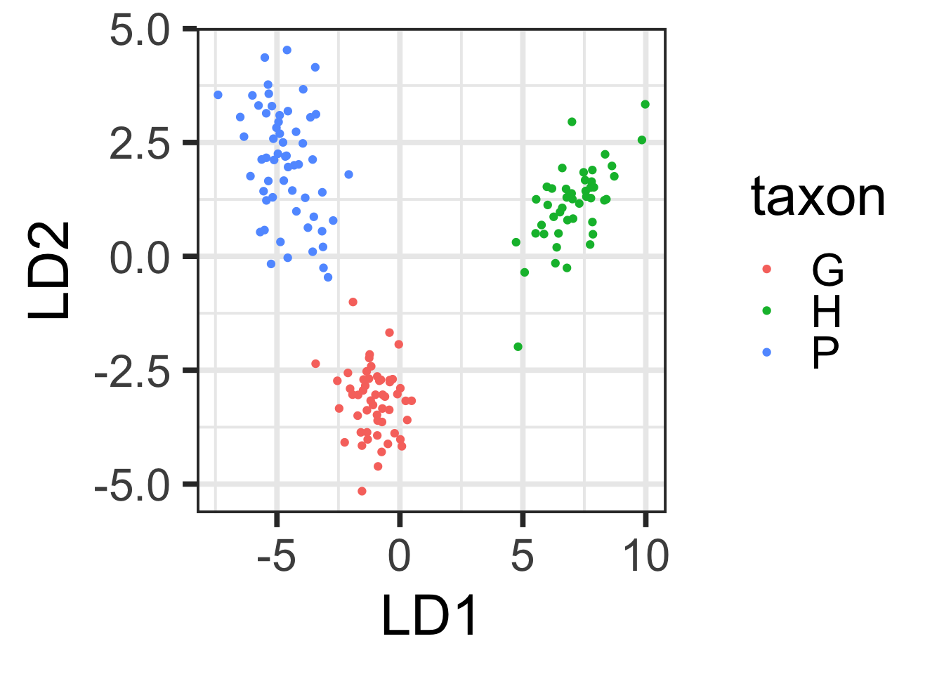

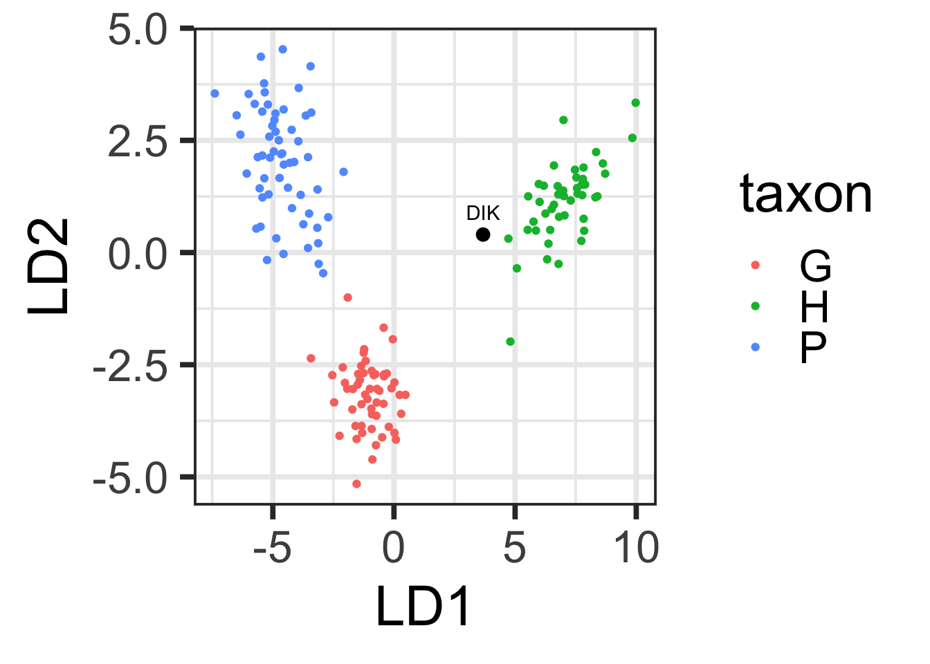
F - 1 bonus pt

Plot the Dikika fossil on the DFA plot.

dikika <- dplyr::filter(scap, Taxon=="D")
DIK_dfa <- predict(DFA, newdata = dikika[,-1])
DIK_plot <- data.frame(DIK_dfa$x, label="DIK")

LDAscatter + 
  geom_point(data=DIK_plot,size=3) + 
  geom_text(data=DIK_plot,aes(x=LD1, y=LD2 + 0.5, label=label))