9 pts total
Problem 1
A - 1pt
howell <- read.table("https://stats.are-awesome.com/datasets/Howell_craniometry.txt", header=TRUE, sep=",")
library(dplyr)
##
## Attaching package: 'dplyr'## The following objects are masked from 'package:stats':
##
## filter, lag## The following objects are masked from 'package:base':
##
## intersect, setdiff, setequal, unionB - 1pt
howell <- howell %>%
  dplyr::select(ID, Sex, Population, BNL, MDH, EKB, ZOR, BAA, NBA) %>%
  dplyr::filter(Population %in% c("BUSHMAN", "PERU", "NORSE", "ZULU"))
head(howell)
## ID Sex Population BNL MDH EKB ZOR BAA NBA
## 1 1 M NORSE 100 31 100 81 39 76
## 2 2 M NORSE 102 19 96 84 35 79
## 3 3 M NORSE 102 28 97 82 38 72
## 4 4 M NORSE 100 25 99 79 46 75
## 5 5 M NORSE 97 26 97 79 42 80
## 6 6 M NORSE 106 29 98 88 39 77C - 1pt
cov(howell[,4:9])## BNL MDH EKB ZOR BAA NBA
## BNL 31.990992 8.122307 15.9348763 21.629802 -1.5687912 -2.261421
## MDH 8.122307 16.495175 5.4709631 3.281787 4.9648033 1.509080
## EKB 15.934876 5.470963 20.0245801 13.425144 -0.6598362 -2.085858
## ZOR 21.629802 3.281787 13.4251439 24.084470 -4.6930390 -6.212397
## BAA -1.568791 4.964803 -0.6598362 -4.693039 11.3239096 3.836069
## NBA -2.261421 1.509080 -2.0858584 -6.212397 3.8360691 10.873610#gives the same results
var(howell[,4:9])## BNL MDH EKB ZOR BAA NBA
## BNL 31.990992 8.122307 15.9348763 21.629802 -1.5687912 -2.261421
## MDH 8.122307 16.495175 5.4709631 3.281787 4.9648033 1.509080
## EKB 15.934876 5.470963 20.0245801 13.425144 -0.6598362 -2.085858
## ZOR 21.629802 3.281787 13.4251439 24.084470 -4.6930390 -6.212397
## BAA -1.568791 4.964803 -0.6598362 -4.693039 11.3239096 3.836069
## NBA -2.261421 1.509080 -2.0858584 -6.212397 3.8360691 10.873610Problem 2
A - 1pt
howellPCA <- prcomp(howell[,4:9], scale=TRUE)
## equivalently, use a formula to specify the variables explicitly
howellPCA <- prcomp(formula = ~ BNL + MDH + EKB + ZOR + BAA + NBA, data=howell, scale=TRUE)
howellPCA
## Standard deviations (1, .., p=6):
## [1] 1.6111576 1.2718569 0.8470599 0.7070900 0.6375459 0.4032368
##
## Rotation (n x k) = (6 x 6):
##            PC1        PC2        PC3         PC4         PC5         PC6
## BNL -0.5491712  0.1353923 -0.2174536  0.03038470  0.45434939 -0.65225549
## MDH -0.2252196  0.5697790  0.4075710  0.65241682 -0.15456185  0.09474583
## EKB -0.5008242  0.1398848 -0.1659344 -0.36470110 -0.75351280 -0.03584305
## ZOR -0.5657892 -0.1237440 -0.0650274 -0.06528556  0.36459373  0.72329154
## BAA  0.1429996  0.6298377  0.3130779 -0.64280335  0.26129312  0.05803093
## NBA 0.2372676 0.4748104 -0.8104439 0.15153822 0.02632561 0.19437863B - 1pt
howellPCA$rotation## PC1 PC2 PC3 PC4 PC5 PC6
## BNL -0.5491712 0.1353923 -0.2174536 0.03038470 0.45434939 -0.65225549
## MDH -0.2252196 0.5697790 0.4075710 0.65241682 -0.15456185 0.09474583
## EKB -0.5008242 0.1398848 -0.1659344 -0.36470110 -0.75351280 -0.03584305
## ZOR -0.5657892 -0.1237440 -0.0650274 -0.06528556 0.36459373 0.72329154
## BAA 0.1429996 0.6298377 0.3130779 -0.64280335 0.26129312 0.05803093
## NBA 0.2372676 0.4748104 -0.8104439 0.15153822 0.02632561 0.19437863ZOR loads strongest on PC1 with a loading of -0.5657892. Note: it is the absolute value that matters here!
C - 1pt
summary(howellPCA)## Importance of components:
## PC1 PC2 PC3 PC4 PC5 PC6
## Standard deviation 1.6112 1.2719 0.8471 0.70709 0.63755 0.4032
## Proportion of Variance 0.4326 0.2696 0.1196 0.08333 0.06774 0.0271
## Cumulative Proportion 0.4326 0.7022 0.8218 0.90516 0.97290 1.0000The cumulative proportion of variance up to and including PC2 is 0.7022
D - 3 pts
forPlot <- data.frame(howellPCA$x, howell$Population)
library(ggplot2)
xAxisLabel <- sprintf("PC1 (%.2f%%)", summary(howellPCA)$importance[2,"PC1"]*100)
yAxisLabel <- sprintf("PC2 (%.2f%%)", summary(howellPCA)$importance[2,"PC2"]*100)
pcPlot <- ggplot(forPlot, aes(x=PC1, y=PC2)) +
  geom_point(size=3,aes(color=howell.Population)) +
  labs(title="PCA of Howell Cranial Measurments",
       color="Population",
       x=xAxisLabel,
       y=yAxisLabel) +
  theme_bw(20) +
  theme(legend.position="top")
pcPlot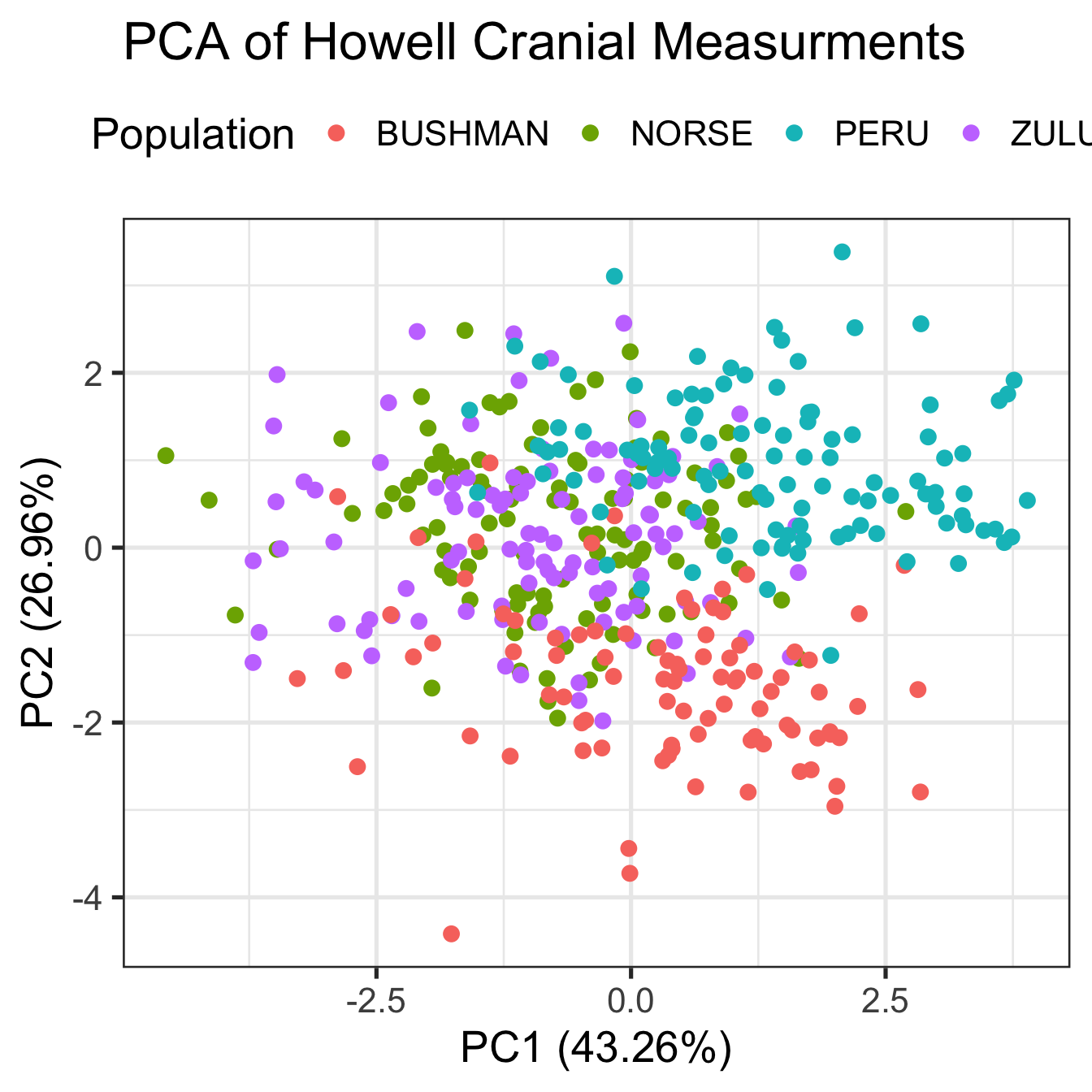
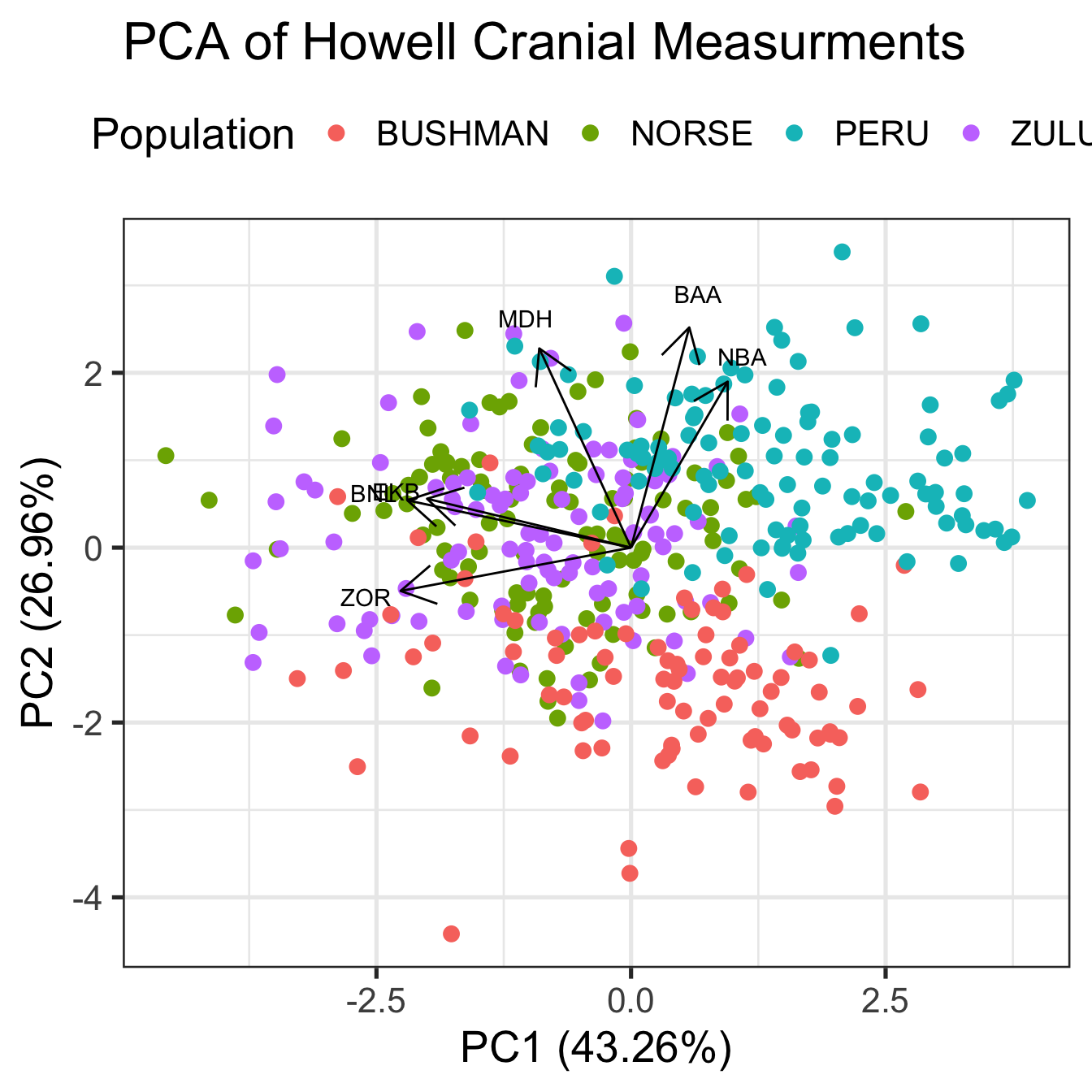
you get a quadruple gold star if you managed to plot the variable loadings on the scatterplot
forLoadings <- data.frame(howellPCA$rotation, x=rep(0, 6), y=rep(0,6), var=rownames(howellPCA$rotation))

scalar <- 4

pcPlot +
  geom_segment(data=forLoadings,
               aes(x=x, y=y, xend=PC1*scalar, yend=PC2*scalar),
               arrow = arrow()) +
  geom_text(data=forLoadings,
            aes(x=PC1*scalar*1.15, y=PC2*scalar*1.15, label=var))