19 points total
Problem 1
A. 1 pt
astrag <- read.table("https://stats.are-awesome.com/datasets/barr_astrag_2014.txt", sep="\t", header=TRUE)B. 2 pt
library(ggplot2)
scatter <- ggplot() +
              geom_point(aes(x=log(B), y=log(DistRad)), data=astrag) +
              labs(title="log(DistRad)~log(B)") +
              theme_bw(20)
scatter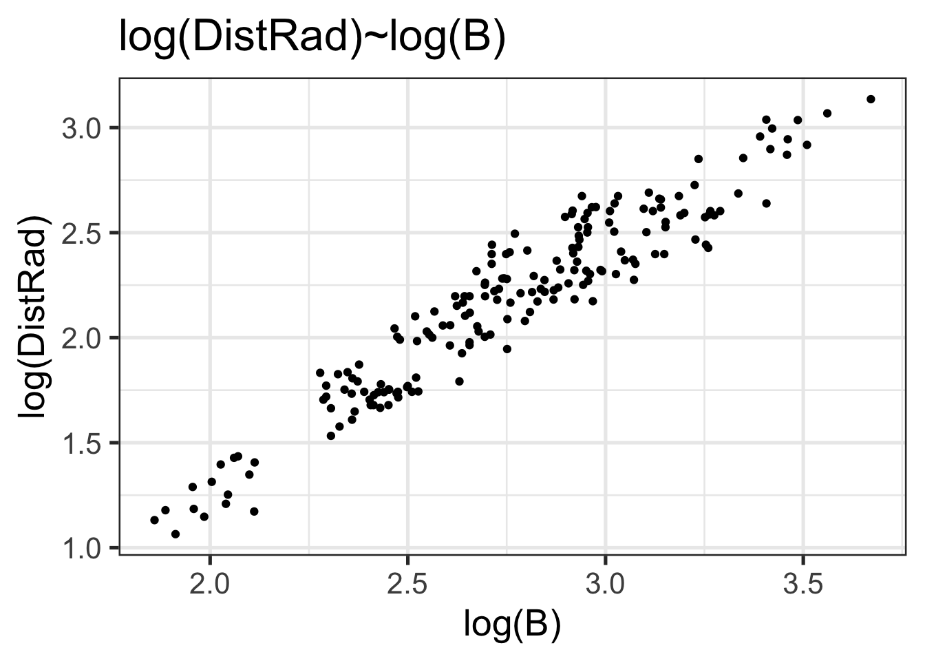
C. 2 pts
OLS_model <- lm(log(DistRad)~log(B), data=astrag)
summary(OLS_model)
##
## Call:
## lm(formula = log(DistRad) ~ log(B), data = astrag)
##
## Residuals:
## Min 1Q Median 3Q Max
## -0.30157 -0.10421 -0.00748 0.09753 0.31963
##
## Coefficients:
## Estimate Std. Error t value Pr(>|t|)
## (Intercept) -0.88445 0.07236 -12.22 <2e-16 ***
## log(B) 1.10855 0.02600 42.63 <2e-16 ***
## ---
## Signif. codes: 0 '***' 0.001 '**' 0.01 '*' 0.05 '.' 0.1 ' ' 1
##
## Residual standard error: 0.1349 on 185 degrees of freedom
## Multiple R-squared: 0.9076, Adjusted R-squared: 0.9071
## F-statistic: 1817 on 1 and 185 DF, p-value: < 2.2e-16D. 3 pts
library(lmodel2)
RMA_model <- lmodel2(log(DistRad)~log(B), data=astrag)
## RMA was not requested: it will not be computed.## No permutation test will be performedRMA_model##
## Model II regression
##
## Call: lmodel2(formula = log(DistRad) ~ log(B), data = astrag)
##
## n = 187 r = 0.9526853 r-square = 0.9076092
## Parametric P-values: 2-tailed = 1.286004e-97 1-tailed = 6.430018e-98
## Angle between the two OLS regression lines = 2.744561 degrees
##
## Regression results
## Method Intercept Slope Angle (degrees) P-perm (1-tailed)
## 1 OLS -0.8844535 1.108552 47.94708 NA
## 2 MA -1.0602519 1.172325 49.53564 NA
## 3 SMA -1.0362204 1.163608 49.32436 NA
##
## Confidence intervals
## Method 2.5%-Intercept 97.5%-Intercept 2.5%-Slope 97.5%-Slope
## 1 OLS -1.027206 -0.7417007 1.057250 1.159854
## 2 MA -1.213964 -0.9145619 1.119474 1.228087
## 3 SMA -1.180755 -0.8979175 1.113436 1.216040
##
## Eigenvalues: 0.3329658 0.007876679
##
## H statistic used for computing C.I. of MA: 0.0005221113E. 1 pts
The OLS slope (1.108552) is less than the RMA slope (1.172325).
F. 3 pts
reg_lines <- data.frame(slopes = c(RMA_model$reg[3,3],coef(OLS_model)[2]),
                        intercepts = c(RMA_model$reg[3,2], coef(OLS_model)[1]), method=c("RMA","OLS")
                        )
withRegLines <- scatter +
  geom_abline(aes(slope=slopes, intercept=intercepts, linetype=method, color=method),
              data=reg_lines, linewidth=2, alpha=0.5)
withRegLines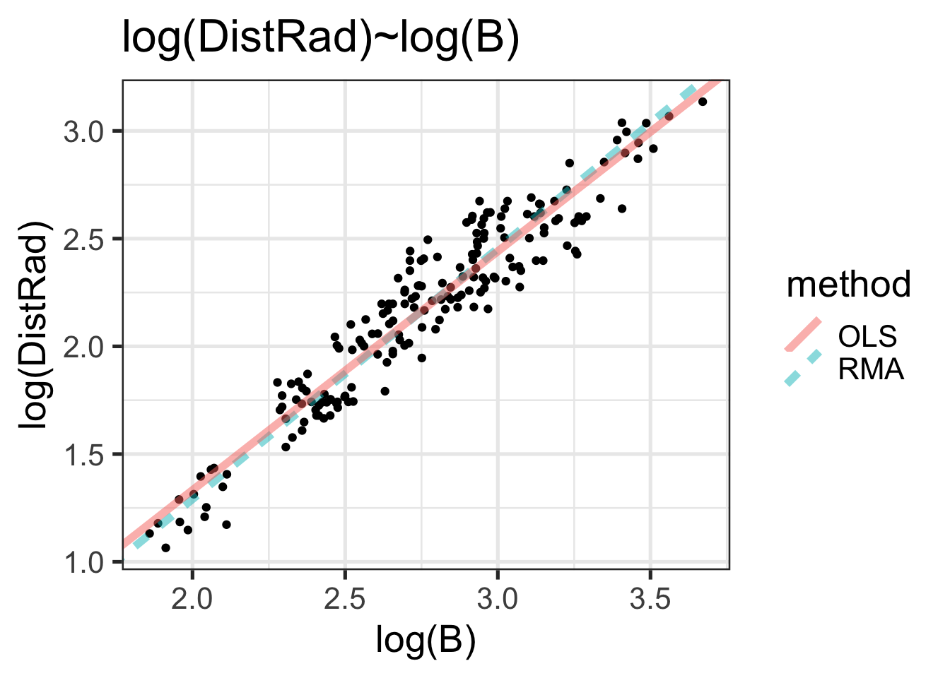
G. 3 pts
plot(OLS_model)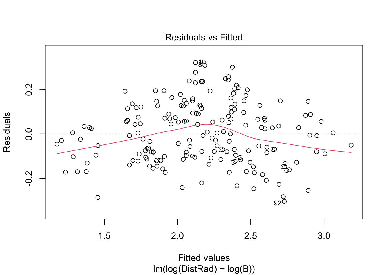
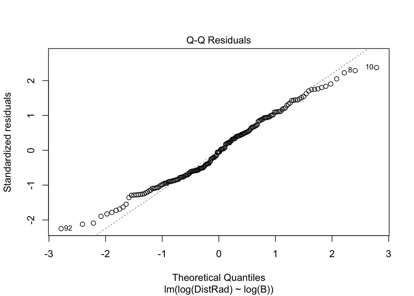
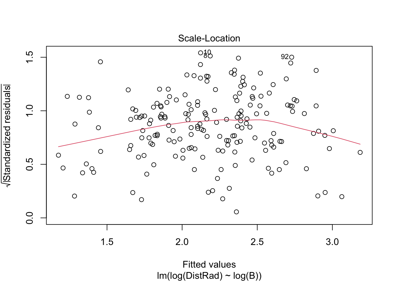
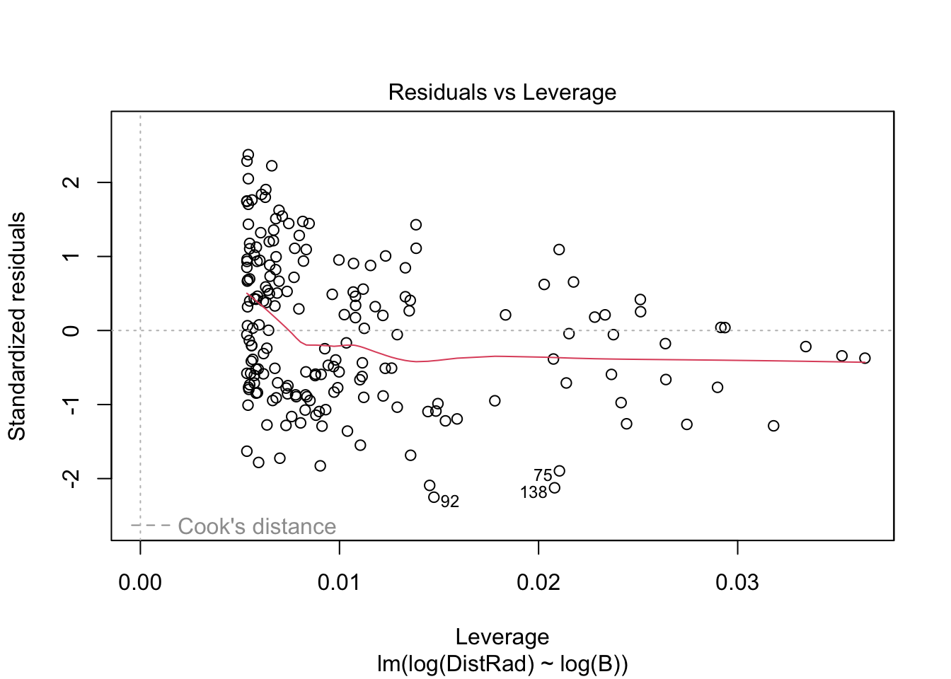
There is evidence that the residuals are not normally distributed.
H. 2pts
qplot(resid(OLS_model), main="Histogram of residuals from OLS") + theme_bw(20)## Warning: `qplot()` was deprecated in ggplot2 3.4.0.
## This warning is displayed once every 8 hours.
## Call `lifecycle::last_lifecycle_warnings()` to see where this warning was
## generated.## `stat_bin()` using `bins = 30`. Pick better value with `binwidth`.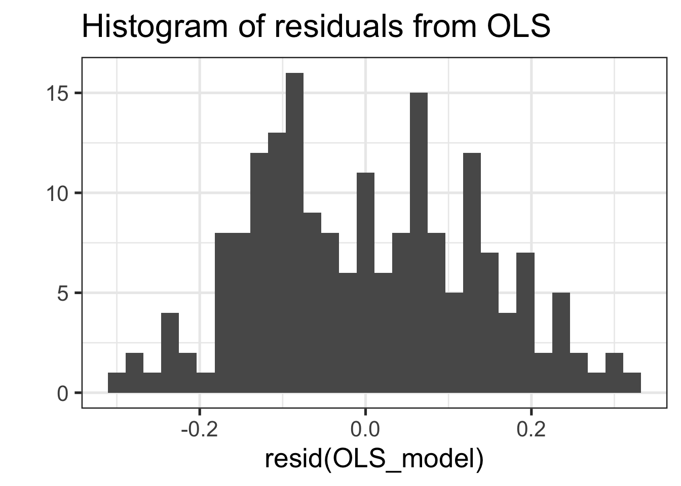
I. 2pts
library(dplyr)
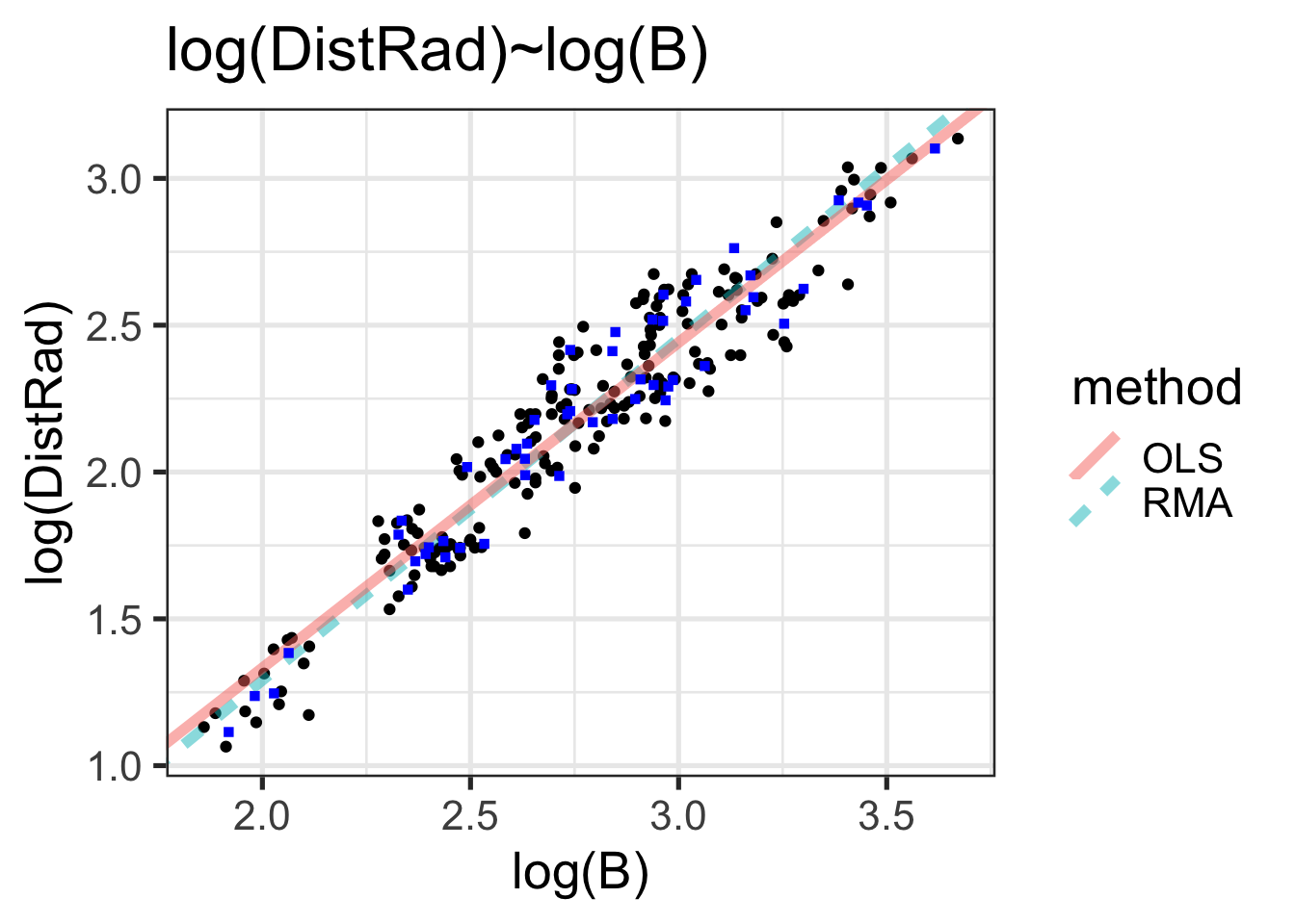
speciesMeans <-
astrag %>%
group_by(Taxon) %>%
summarize(logB=mean(log(B), na.rm=T), logDistRad=mean(log(DistRad), na.rm=T))
withRegLines +
geom_point(aes(x=logB, y=logDistRad), data=speciesMeans, color="blue", shape=15)