Homework # 4 - Solution

part A - 2pts

foots <- read.table("https://stats.are-awesome.com/datasets/american_feet.txt", header=TRUE)
library(ggplot2)

thePlot <- ggplot(foots, aes(x=height, y=foot_length)) +
  labs(x="height(cm)",
       y="foot length(cm)",
       title="foot length by height in simulated americans") + 
  geom_point() 

thePlot +  
  stat_smooth(method="lm") + 
  theme_bw(18)

## `geom_smooth()` using formula = 'y ~ x'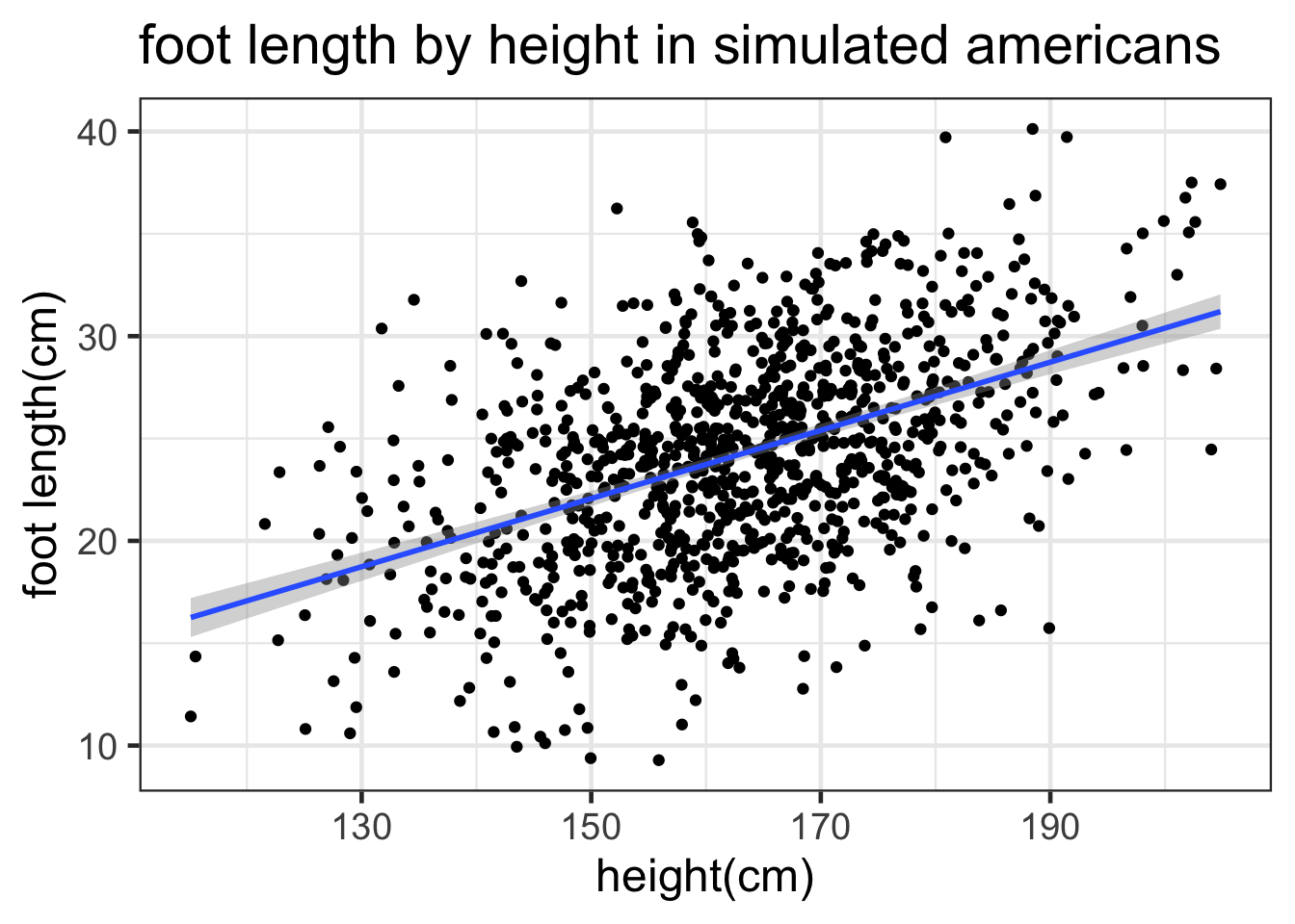

part B - 2pts

cors <- numeric(10000)
for(each in 1:10000){
  cors[each] <- abs(cor(foots$height, sample(foots$foot_length)))
}

part C - 1pt

## ggplot demands a dataframe, so we first change our vector into a dataframe
cors <- as.data.frame(cors)

ggplot(cors, aes(x=cors)) + 
  geom_histogram(color="white") + 
  labs(x="absolute value of correlation coefficient",
       title="test statistics from 10,000 iterations") + 
  theme_bw(18)

## `stat_bin()` using `bins = 30`. Pick better value with `binwidth`.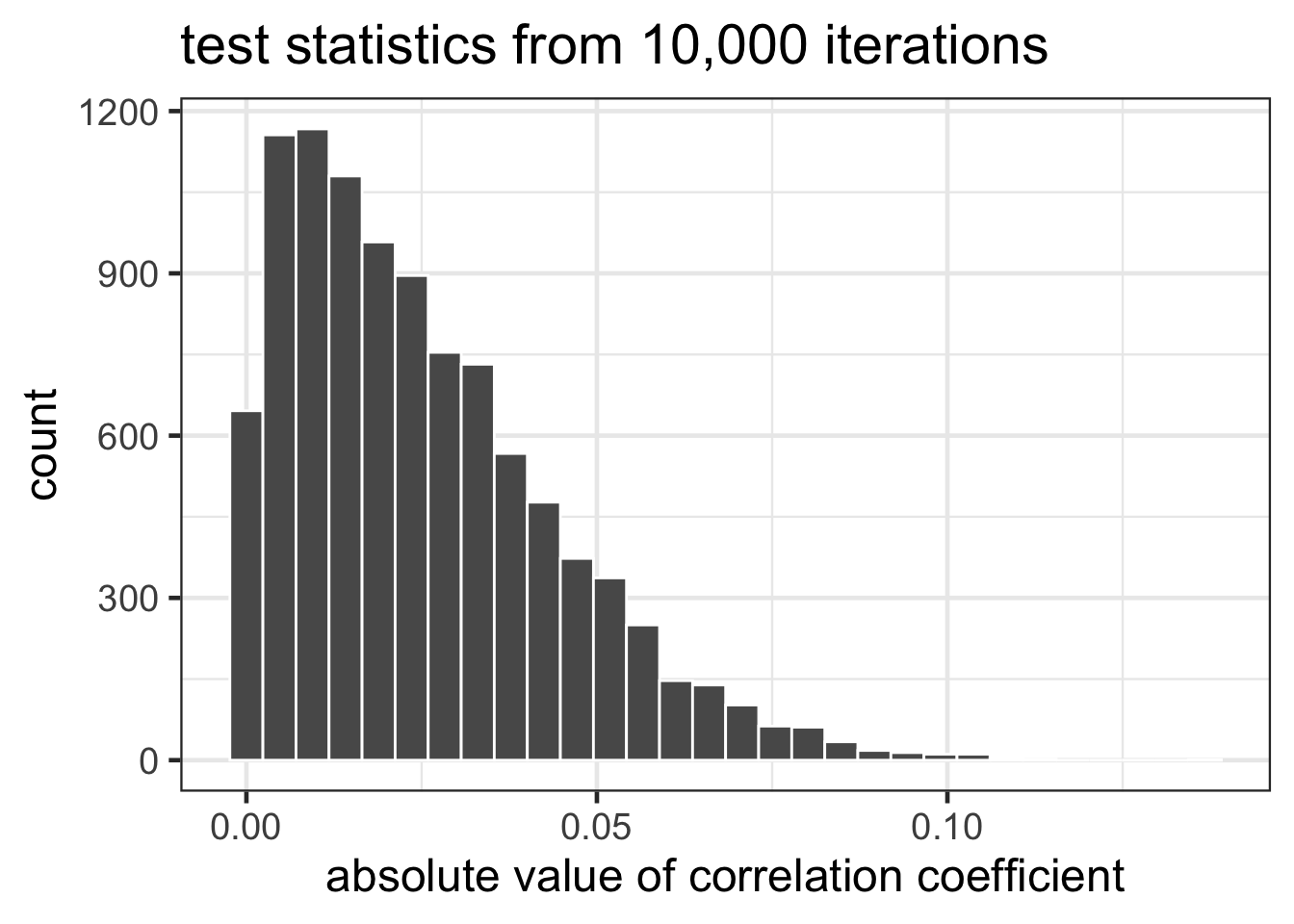

part D - 1pt

original.cor <- abs(cor(foots$foot_length, foots$height))
original.cor

## [1] 0.4776426

part E - 1pt

sum(cors>=original.cor) / length(cors)

## [1] 0

part F - 2pts

Our set of 10,000 reshuffled vectors represented the null hypothesis in which there was no systematic relationship between height and foot length. None of the test statistics computed on reshuffled data was as extreme as our observed test statistic on the unshuffled data. Thus, we should reject the null hypothesis and conclude that there is a relationship between the two variables.

3 points

In parametric statistics, the null hypothesis is specified by hypothetical mathematical distributions of test statistics (e.g. the F-distribution), and estimating the tail probability of an observed test statistic with respect to the null distribution. Since the mathematical distribution is defined from -∞ to ∞, the tail probability of any observed test statistic will be non-zero, no matter how extreme. So, a p-value of zero is not possible.

In Monte Carlo statistics, the null hypothesis is specified by randomizing the dataset. Since the null distribution is estimated in this way, there are only a finite number of ways to re-shuffle the dataset. It is possible that none of the reshufflings will be as extreme as the observed test statistic resulting in a p-value of zero. Keep in mind that as additional data are collected, then the null distribution will change.