Homework # 3 - Solution

Part A

Note that columns 1 thorough 4 are the numeric columns in the iris dataset.

for(i in 1:4){
  print(shapiro.test(iris[,i])$p.value)
}

## [1] 0.01018116
## [1] 0.1011543
## [1] 7.412263e-10
## [1] 1.680465e-08

Part B

library(ggplot2)
qplot(iris$Sepal.Length) 

## Warning: `qplot()` was deprecated in ggplot2 3.4.0.
## This warning is displayed once every 8 hours.
## Call `lifecycle::last_lifecycle_warnings()` to see where this warning was
## generated.

## `stat_bin()` using `bins = 30`. Pick better value with `binwidth`.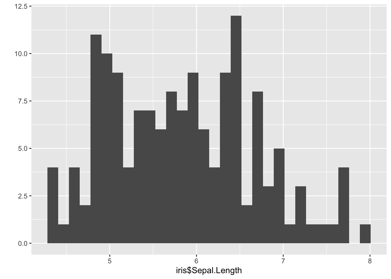

qplot(iris$Sepal.Width) 

## `stat_bin()` using `bins = 30`. Pick better value with `binwidth`.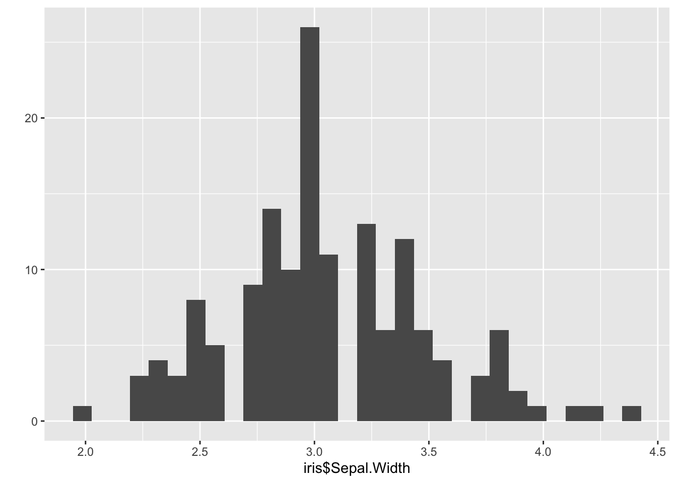

qplot(iris$Petal.Length) 

## `stat_bin()` using `bins = 30`. Pick better value with `binwidth`.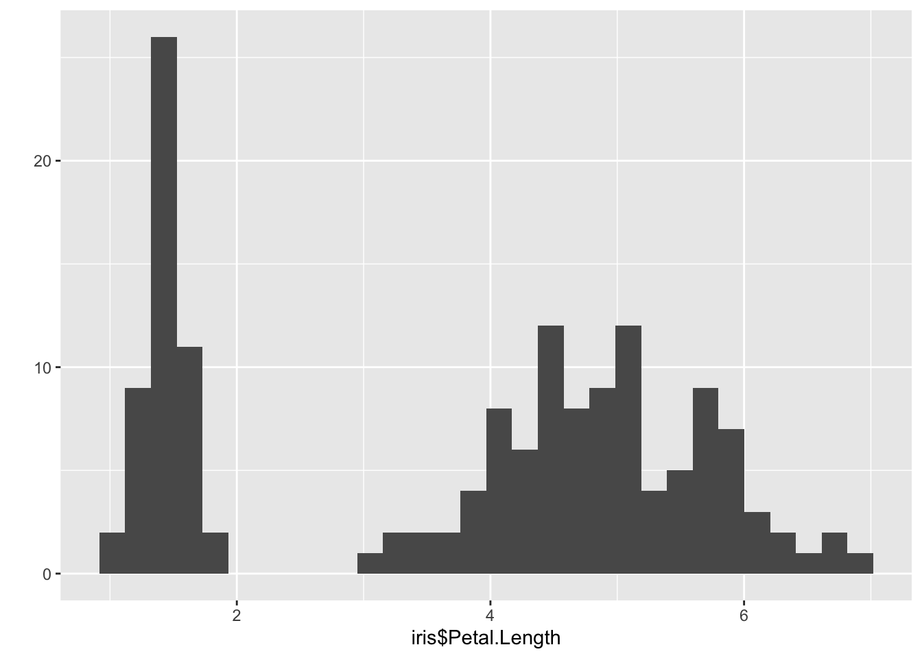

qplot(iris$Petal.Width) 

## `stat_bin()` using `bins = 30`. Pick better value with `binwidth`.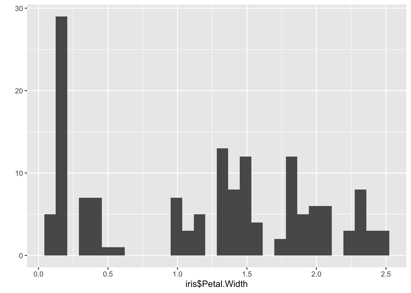

Part D

mean(iris$Sepal.Length^2)

## [1] 34.82567

median(iris$Sepal.Length^2)

## [1] 33.64

Part E

These values are different because the distribution of iris$Sepal.Length^2 is asymmetric, as shown in the below histogram.

qplot(iris$Sepal.Length^2)

## `stat_bin()` using `bins = 30`. Pick better value with `binwidth`.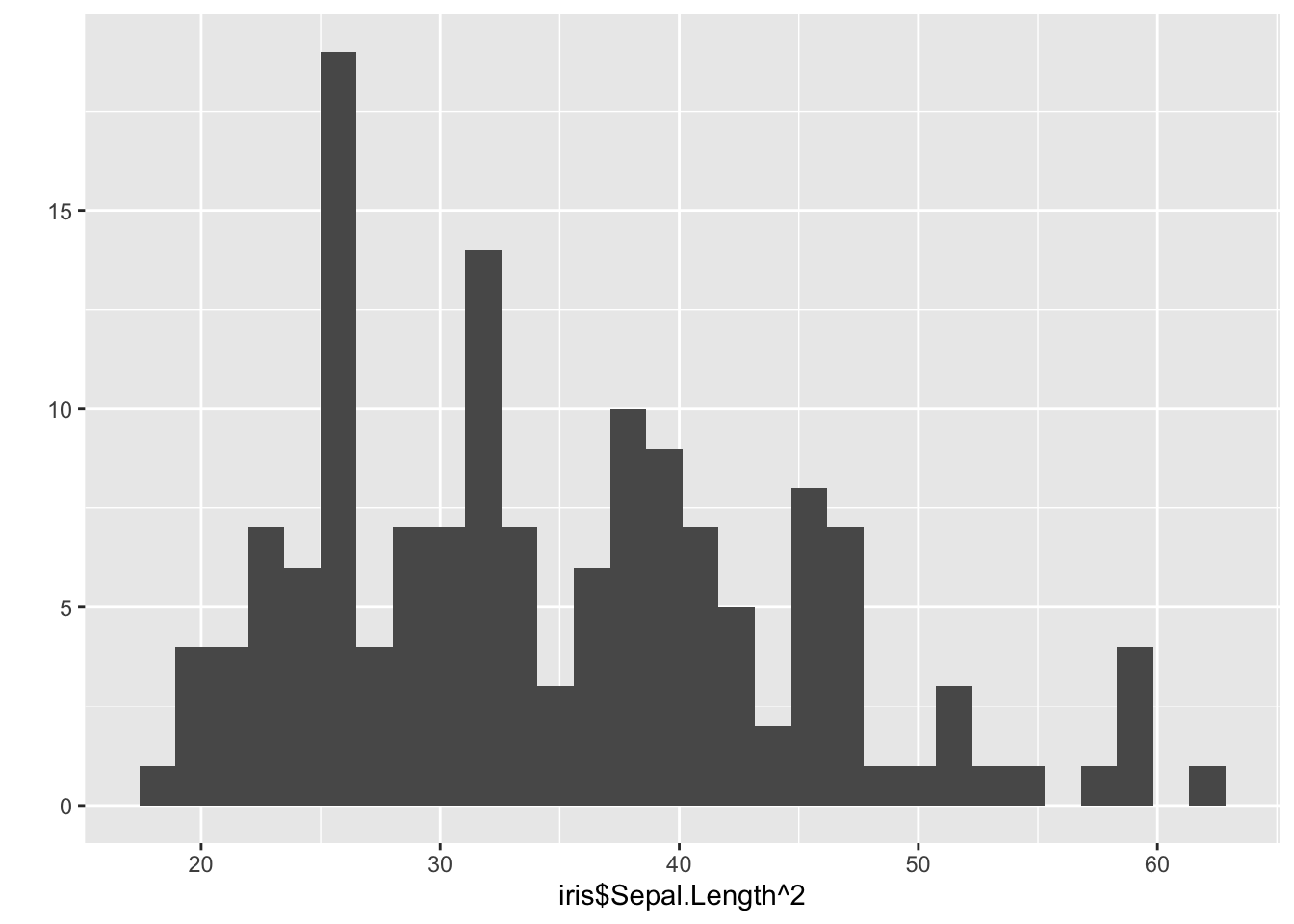

The distribution has a long right tail, which heavily influences the mean, pulling it towards the larger values. The median is less affected by extreme values.

Part A

filez <- list.files("/Path/to/folder", full=TRUE)

Set up and run a for() loop

# create empty vector, to be filled up with the averages
proportions_of_G <- rep(NA,100)

#loop through index numbers of files

for(i in 1:length(filez)){
  #read file in
  df <- read.table(filez[i], header=T, sep=",")
  #calculate the proportion of G
  propG <- sum(df$base == "G") / length(df$base)
  #update the results vector with the proportion from current file
  proportions_of_G[i] <- propG
}

Alternatively, you could do it with sapply() and a custom function. Note: the difference between lapply() and sapply() whether you get a list or a vector as a result (l stand for list).

doIt <- function(filename){
  df <- read.table(filename, header=T, sep=",")
  propG <- sum(df$base == "G") / length(df$base)
  return(propG)
}
proportions_of_G <- sapply(filez, doIt)

After running the for loop, we can report the average proportion of G across all files

mean(proportions_of_G)

## [1] 0.2491692

Part B

library(ggplot2)
ggplot(mapping=aes(x=proportions_of_G)) + 
  geom_histogram(bins=10) + 
  labs(x="Proportion of G", 
       title="Proportions of Guanine across 100 genetic sequences")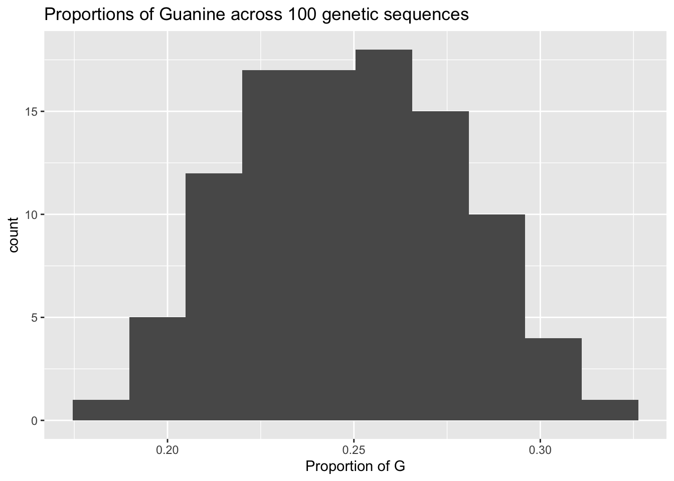

Part C

This is a decently normal distribution. It is fairly symmetrical around the mean…its pretty unimodal. If we want to put a number on our intuition, the shapiro.test() agrees it is normal.

shapiro.test(proportions_of_G)

## 
## 	Shapiro-Wilk normality test
## 
## data:  proportions_of_G
## W = 0.99236, p-value = 0.8469