Homework #2 - Solution

5 points possible

• 1 pt reorder factor
• 1 pt fill color
• 1 pt legend
• 1 pt title
• 1 pt theme

library(ggplot2)
chickwts$feed <- reorder(chickwts$feed, chickwts$weight, median)
ggplot(chickwts, aes(x=feed, y=weight)) +   
  geom_boxplot(aes(fill=feed)) + 
  scale_fill_brewer(palette="Blues") + 
  labs(title="Chick weights on different diets", x="feed type", y="weight(g)") + 
  theme_bw(14)

5 points possible

1. 2 pt means
2. 3 pts figure

Part a

library(dplyr)

## 
## Attaching package: 'dplyr'

## The following objects are masked from 'package:stats':
## 
##     filter, lag

## The following objects are masked from 'package:base':
## 
##     intersect, setdiff, setequal, union

crania <- read.table("https://stats.are-awesome.com/datasets/Howell_craniometry.txt",sep=",", header=TRUE, na.strings = '0')

crania %>% 
  group_by(Population, Sex) %>%
  summarise(meanGOL = mean(GOL), meanXCB = mean(XCB), meanZYB=mean(ZYB), meanSIS = mean(SIS))

## `summarise()` has grouped output by 'Population'. You can override using the
## `.groups` argument.

## # A tibble: 56 × 6
## # Groups:   Population [30]
##    Population Sex   meanGOL meanXCB meanZYB meanSIS
##    <chr>      <chr>   <dbl>   <dbl>   <dbl>   <dbl>
##  1 AINU       F        179.    137.    128.    2.78
##  2 AINU       M        190.    143.    139.    3.65
##  3 ANDAMAN    F        160.    131.    118.    2.17
##  4 ANDAMAN    M        169.    136.    124.    2.33
##  5 ANYANG     M        181     139.    136.    2.37
##  6 ARIKARA    F        171.    136.    131.    3.47
##  7 ARIKARA    M        179.    142.    141.    4.25
##  8 ATAYAL     F        168.    132.    124.    2.43
##  9 ATAYAL     M        177.    136.    133.    2.85
## 10 AUSTRALI   F        181.    128.    126.    3.47
## # ℹ 46 more rows

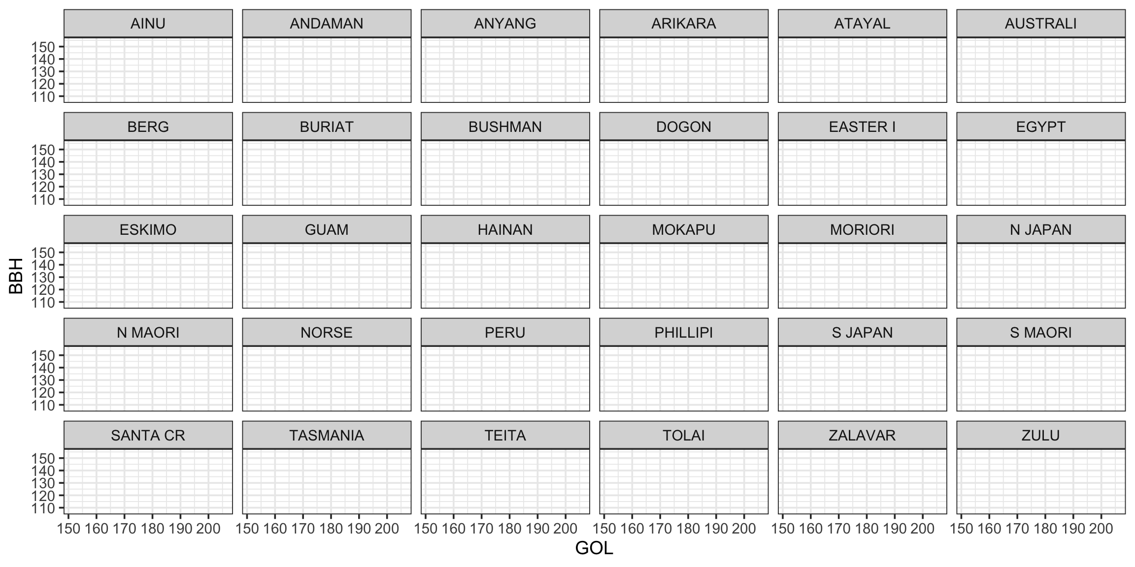
Part b

library(ggplot2)
ggplot(data=crania, mapping=aes(x=GOL, y=BBH)) + 
  facet_wrap(vars(Population)) + 
  theme_bw(14)