1. Indexing Vectors
5 points possible
- 1pt length
- 1pt first four
- 1pt last 8
- 1pt various
- 1pt reverse
nouns <- c("apple", "flower", "insect", "lettuce", "knife", "dog", "cloud", "person", "cabinet", "flower" )

#length
length(nouns)
## [1] 10#first four
nouns[1:4]## [1] "apple" "flower" "insect" "lettuce"#last 8
nouns[3:10]## [1] "insect" "lettuce" "knife" "dog" "cloud" "person" "cabinet"
## [8] "flower"#various elements
nouns[c(1, 3:6, 10)]## [1] "apple" "insect" "lettuce" "knife" "dog" "flower"#reverse
nouns[10:1]## [1] "flower" "cabinet" "person" "cloud" "dog" "knife" "lettuce"
## [8] "insect" "flower" "apple"#alternate reverse
rev(nouns)## [1] "flower" "cabinet" "person" "cloud" "dog" "knife" "lettuce"
## [8] "insect" "flower" "apple"2. Using functions
7 points possible
- 1pt grades
- 1pt curve
- 1pt sd
- 1pt min
- 1pt max
- 1pt mean
- 1pt hist
grades <- rnorm(200, mean = 68, sd=10)

#curve
curvedgrades <- grades + 7
curvedgrades
## [1] 71.14957 79.73831 72.11741 63.99216 66.33171 87.01095 85.28948
## [8] 77.71542 69.31031 82.21867 69.87873 81.04276 85.59338 57.41413
## [15] 77.21444 77.36932 78.33611 76.56771 65.41453 67.29659 69.12338
## [22] 72.87651 83.29551 62.49451 68.99733 89.39655 64.23113 80.06728
## [29] 67.75579 76.58815 84.59640 74.80297 77.92369 77.03485 89.63609
## [36] 79.01616 47.04780 62.54018 82.61821 74.91004 71.11674 71.57571
## [43] 82.00167 78.55127 81.06247 83.26583 69.49709 77.04976 79.01556
## [50] 75.99059 66.29371 71.50357 87.27525 68.13417 68.28725 84.99742
## [57] 65.10828 83.87751 61.60146 72.45147 58.38770 89.20695 68.59041
## [64] 94.38511 76.26781 74.47974 64.74157 78.14960 84.51308 58.53508
## [71] 80.30772 66.96190 70.66336 77.84683 80.58597 89.97218 72.40484
## [78] 80.46092 85.69119 73.78970 85.40264 64.53390 73.97515 74.68257
## [85] 79.96900 71.94004 76.57589 84.14442 87.93350 88.48653 67.34533
## [92] 70.55957 61.31363 71.93250 48.98816 75.50367 91.08383 66.60164
## [99] 76.97148 75.69569 69.81478 83.32165 80.57704 89.07246 68.21824
## [106] 86.01700 57.37012 76.44270 75.26520 80.23017 83.33712 84.20003
## [113] 77.63815 68.00980 77.12992 79.33750 76.31992 64.79642 61.76321
## [120] 69.33234 83.33258 80.03076 86.02090 84.87266 76.26466 75.37907
## [127] 65.47466 81.17607 62.77789 66.78656 80.26604 71.43315 90.53552
## [134] 78.98691 77.21292 73.80357 76.32166 72.11558 68.57404 58.77041
## [141] 74.93604 73.96505 76.60968 86.59149 69.72317 71.63764 81.83682
## [148] 79.53350 70.16158 62.02626 86.14184 76.41898 90.39728 85.84489
## [155] 59.99313 61.95783 76.65714 78.25780 84.18816 58.30453 71.68278
## [162] 60.24773 83.37843 76.15287 70.98476 70.70184 67.08870 70.25938
## [169] 56.50525 66.06198 74.39020 97.21465 72.14294 100.03358 88.00999
## [176] 84.53187 73.65474 82.24849 73.05010 73.55741 78.09537 73.47364
## [183] 77.74656 58.00107 83.68196 76.06975 72.35222 89.07631 74.42315
## [190] 81.17216 78.37786 72.33805 68.34523 62.60553 75.99556 71.23971
## [197] 89.42669 48.26760 90.15344 83.56841sd(curvedgrades)## [1] 9.218072min(curvedgrades)## [1] 47.0478max(curvedgrades)## [1] 100.0336mean(curvedgrades)## [1] 75.17006hist(curvedgrades)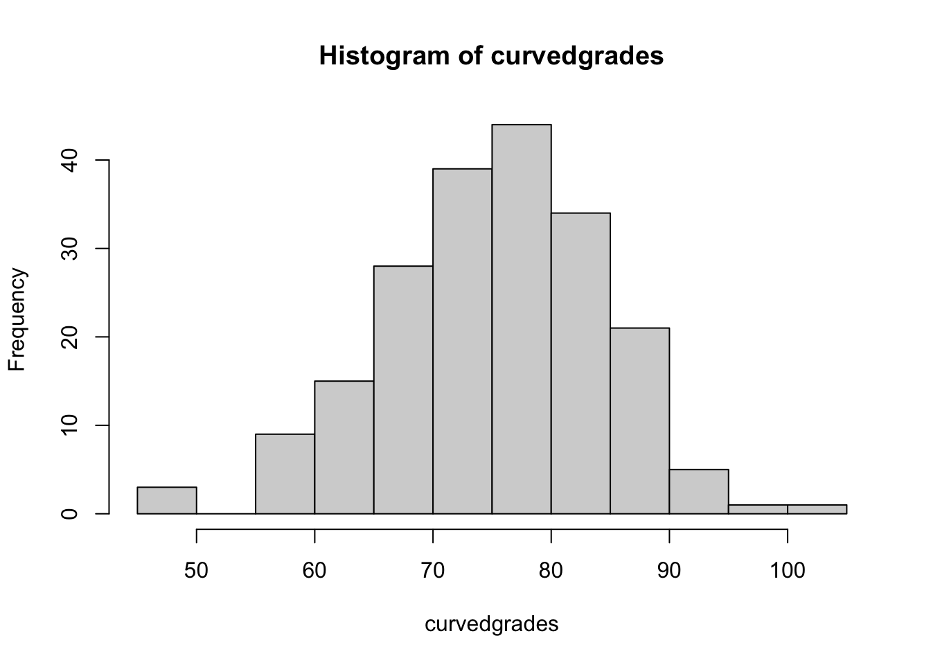
3. Organizing data
4 points possible
- 2pts - fix data
- 2pts - describe problems
The original data file had duplicated column names (length and diameter), relying on another column to differentiate the anatomical element. This is a no, no. Column names must stand alone (e.g. tibia_diameter).
The rows containing species names violate the 1 row = 1 observation priciple. These rows should be turned into a column which records the species for each observation.
4. Manipulation
7 pts possible
- 1pt gorilla
- 2pts sex
- 1pt table
- 1pt hist
- 1pt small
- 1pt big
gorilla <- read.table("https://stats.are-awesome.com/datasets/gorilla_sizes.txt", header=TRUE)

#figure out sex


## do it with grepl
isMale <- factor(grepl("m", gorilla$specimen))
#rename the trues and falses by updating the labels for each factor level
levels(isMale) <- c("female", "male")
gorilla$sex <- isMale

#alternate way - first make a new column which will keep track of sex, with 59 NA values as a placeholder
gorilla$sex <- rep(NA, 59)

# now replace the NA values with 'Male' or 'Female' with the help of grep()
gorilla$sex[grep("m", gorilla$specimen)] <- "Male"
gorilla$sex[grep("f", gorilla$specimen)] <- "Female"


table(gorilla$sex)
##
## Female Male
## 30 29hist(log(gorilla$skull))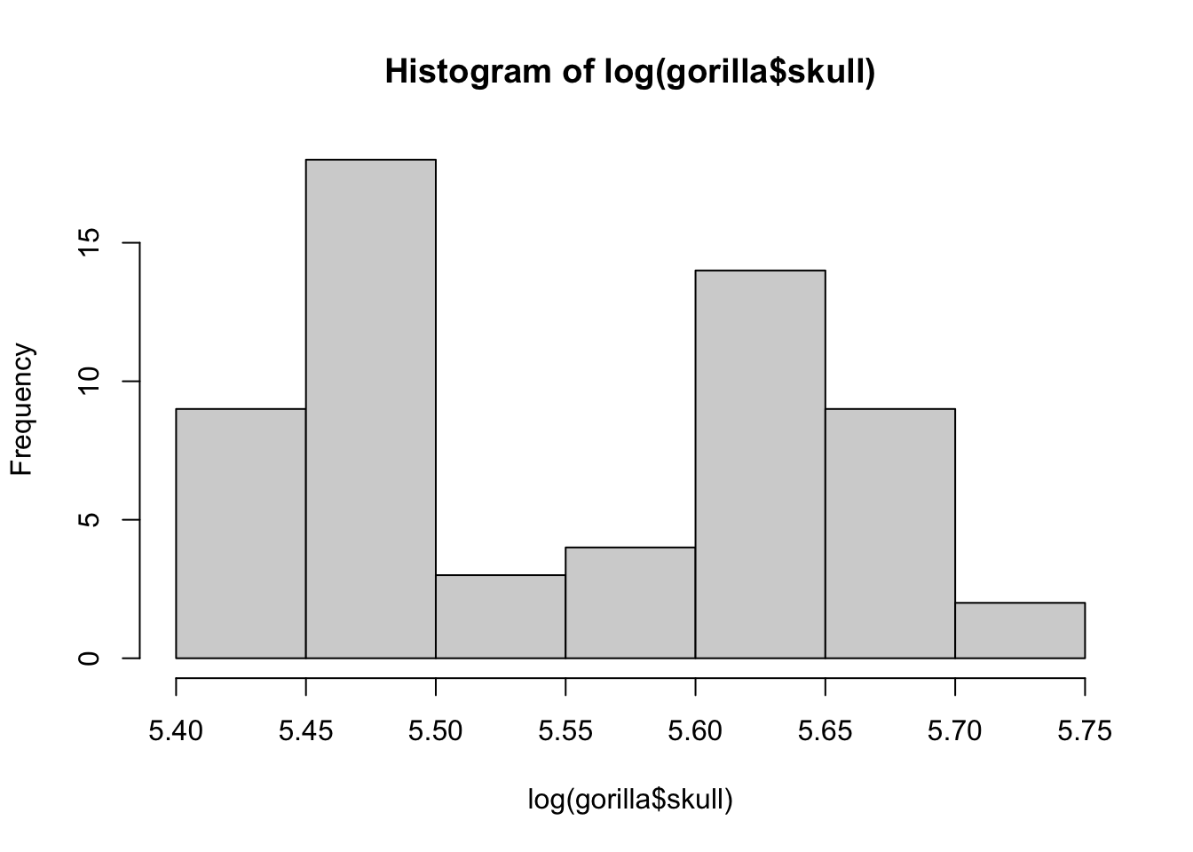
smalls <- gorilla[gorilla$skull < 250,]
smalls
## specimen skull sex
## 1 _0_f1 235.180 Female
## 2 _0_f2 238.968 Female
## 3 _0_f3 235.168 Female
## 4 _0_f4 242.873 Female
## 5 _0_f5 229.244 Female
## 6 _0_f6 240.477 Female
## 7 _0_f7 242.761 Female
## 8 _0_f8 240.322 Female
## 9 _0_f9 237.948 Female
## 10 _0_f10 224.605 Female
## 11 _0_f11 243.091 Female
## 12 _0_f12 240.709 Female
## 13 _0_f13 241.155 Female
## 14 _0_f14 231.046 Female
## 15 _0_f15 228.324 Female
## 16 _0_f16 228.183 Female
## 17 _0_f17 246.153 Female
## 18 _0_f18 228.614 Female
## 19 _0_f19 236.424 Female
## 20 _0_f20 243.491 Female
## 21 _0_f21 229.924 Female
## 22 _0_f22 236.198 Female
## 23 _0_f23 238.134 Female
## 24 _0_f24 238.700 Female
## 25 _0_f25 244.689 Female
## 26 _0_f26 227.045 Female
## 27 _0_f27 232.538 Female
## 28 _0_f28 245.203 Female
## 29 _0_f29 240.910 Female
## 30 _0_f30 245.259 Femalebigs <- subset(gorilla, subset = skull>250)
bigs## specimen skull sex
## 31 _1_m1 270.137 Male
## 32 _1_m2 273.371 Male
## 33 _1_m3 292.082 Male
## 34 _1_m4 276.194 Male
## 35 _1_m5 282.821 Male
## 36 _1_m6 261.352 Male
## 37 _1_m7 267.413 Male
## 38 _1_m8 286.614 Male
## 39 _1_m9 288.243 Male
## 40 _1_m10 287.369 Male
## 41 _1_m11 275.070 Male
## 42 _1_m12 302.074 Male
## 43 _1_m13 280.033 Male
## 44 _1_m14 276.853 Male
## 45 _1_m15 273.564 Male
## 46 _1_m16 287.930 Male
## 47 _1_m17 273.241 Male
## 48 _1_m18 271.774 Male
## 49 _1_m19 287.890 Male
## 50 _1_m20 296.964 Male
## 51 _1_m21 283.813 Male
## 52 _1_m22 279.941 Male
## 53 _1_m23 300.346 Male
## 54 _1_m24 291.276 Male
## 55 _1_m25 262.899 Male
## 56 _1_m26 275.778 Male
## 57 _1_m27 276.420 Male
## 58 _1_m28 280.518 Male
## 59 _1_m29 286.621 Male